Differential Abundance Testing
Having a study design in with there are two (or more) groups of samples, say male/female, diet1/diet2, etc. one is often interested in knowing:
- Is there a difference between the groups?
- Which bacteria / OTUs are most different between the groups?
This concept is within microbiome statistics refered to as Differential Abundance Testing.
The principal behind is very simple: Given an OTU matrix of p different OTUs;
Perform p univariate tests assigning an effect size and a p-value to each OTU on the question of differential abundance. That could for example be based on a simple t-test
Arrange the p tests according to the p-value going from the smallest (most different OTU) to the largest (least different OTU)
Deside a cut point for which OTUs to be assigned discoveries. I.e. OTUs with p-values below \(p_{cut}\) to be discoveries. This task is known as multiple-testing-correction, and is a general statistical concept.
Given that todays microbiome studies generates a large number of OTUs, p often higher than 1.000 there are two concerns:
- Choose a reliable and powerful univariate model
- Boost the discovery chance by filter and/or aglommeration
The paper by Thorsen et al 2016 investigates a range of statistical strategies on both the ability to sort the OTUs from the most discriminatory to the least, as well as the false discovery rate control. Russel et al (2019) have streamlined this approach for selecting the relevant statistical engine, which nicely screens +20 methods in very few lines of code (see DAtest for code)
(see refs below)
1 Exercise
1.1 Setting up data
Rarefy the mice birth mode data to even depth, and use the phyloseq_to_deseq2() function to convert format including birht mode as class information.
1.2 DEseq
Perform DA test using DESeq() from the DESeq2 library. You might need to install this library in advance.
library(phyloseq)
library(DESeq2)
load('./data/Mice_csec.RData')

birhtmode_ds <- phyloseq_to_deseq2(phyX, ~ Birth_mode)

res <- DESeq(birhtmode_ds, test="Wald", fitType="parametric")
1.3 Interpret results
Extract results and combine with tax information (from tax_table()) as well as read frequency per OTU as well as presence/absence percentage.
tb <- results(res, cooksCutoff = FALSE)
txtb <- data.frame(tax_table(phyX))

abu <- taxa_sums(phyX)
presence <- apply(otu_table(phyX)>0,1,sum)

df_res <- data.frame(est = tb$log2FoldChange, se = tb$lfcSE, pv = tb$pvalue, pvadj = tb$padj, abu, presence)
df_res <- cbind(df_res, txtb)
df_res$name <- rownames(df_res)
1.4 Is this different from null?
Plot a histogram of the unadjusted p-values. How should this plot look like if there were no birth mode information in the data?
1.5 Vulcano plot
Plot a vulcano plot of the results. Try to facet out / or color according to a taxonomic level to get deeper insight on which bacteria that are affected the most.
ggplot(data = df_res, aes(est,-log10(pv), color = Rank4)) +
  geom_point() +
  geom_text(data = df_res[df_res$pv<0.0001,], aes(label = name), color = 'black') + # put label on the top stuff
  theme(legend.position = 'none') +
  facet_wrap(~Rank3)
1.6 rare/common vs difference
Interpret the results as a function of read-frequency or presence/absence. Is it the dominating species that are most different?
1.7 Effect of agglomoration
Perform tax glommeration (tax_glom()) at some taxonomic level, and re-run the analysis. Do you get the same results?
1.8 Metagenomeseq
Do exactly the same just using t-test, wilcox tests as well as metagenomeseq’s featureModel() and compare the results? Below are some code-inspiration.
library(tidyverse)
library(broom)
library(metagenomeSeq)
mgsdata <- phyloseq_to_metagenomeSeq(phyX)
mgsdata <- cumNorm(mgsdata, p=.5)
mod <- model.matrix(~1+Birth_mode, data=pData(mgsdata))
mgsfit <- fitFeatureModel(obj = mgsdata,mod = mod)

predictor <- sample_data(phyX)$Birth_mode
# do some preprocessing
count_table <- log(t(otu_table(phyX)) + 1)
count_table <- apply(count_table, 2, function(x) x/sum(x))

# use tidyverse and broom to get test
tb_ttest <- count_table %>%
  cbind(predictor) %>%
  data.frame() %>%
  gather(otu,ra,-predictor) %>%
  group_by(otu) %>%
  do(t.test(data = ., ra~predictor) %>% tidy)
allres <- bind_rows(
data.frame(estimate = mgsfit@fitZeroLogNormal$logFC,
p.value = mgsfit@pvalues,
otu = mgsfit@taxa,
test = 'metagenomeseq'),
data.frame(estimate = tb$log2FoldChange,
p.value = tb$pvalue,
otu = rownames(tb),
test = 'DESeq2'),
tb_ttest %>% mutate(test = 't-test')
)
#plot it!
ggplot(data = allres, aes(estimate,-log10(p.value), label = otu)) +
geom_point() +
geom_text(data = allres[allres$p.value<10e-7 & !is.na(allres$p.value),]) +
facet_wrap(~test,nrow = 1, scales = 'free_x')
1.9 Put infeerence on the phylogentic tree
Because the number of taxa is larger, we restrict the plot to include the once with a somewhat significant signal.
library(ggtree)
# Filter object and inference data.
dfsel <- df %>%
  dplyr::filter(pv_MGS<0.1) %>%
  dplyr::mutate(logFC = ifelse(abs(est_MGS)>1.5, sign(est_MGS)*1.5,est_MGS))

phyobj <- phyX %>%
  subset_taxa(rownames(phyX@tax_table) %in% rownames(dfsel))  # this way to make sure it is not depend on order.

TREE <- phy_tree(phyobj)
TXtab <- as.data.frame(tax_table(phyobj))
# merge on inferential stats
AA <- TXtab %>% rownames_to_column('otu') %>%
  left_join(dfsel%>% rownames_to_column('otu') , by = 'otu')
# initiale tree
g3 <- ggtree(TREE,layout = 'circular',branch.length="none")
g3 <- g3 %<+%  AA
g3 <- g3 +
  geom_tippoint(aes(x = x+1, fill = logFC, subset = isTip), shape=21,size = 2 )  +
  # geom_text(aes(label = node)) + # use this to get node numbers, and then apply in geom_highlight
  geom_hilight(node=1038, fill="gray10", alpha=.2) +
  scale_fill_gradient2(low = 'red',high = 'darkgreen',
                       midpoint = 0,mid = 'white',
                       na.value = 'grey95',
                       name = 'logFC')  +
  theme(legend.position="right",legend.title=element_blank())
g3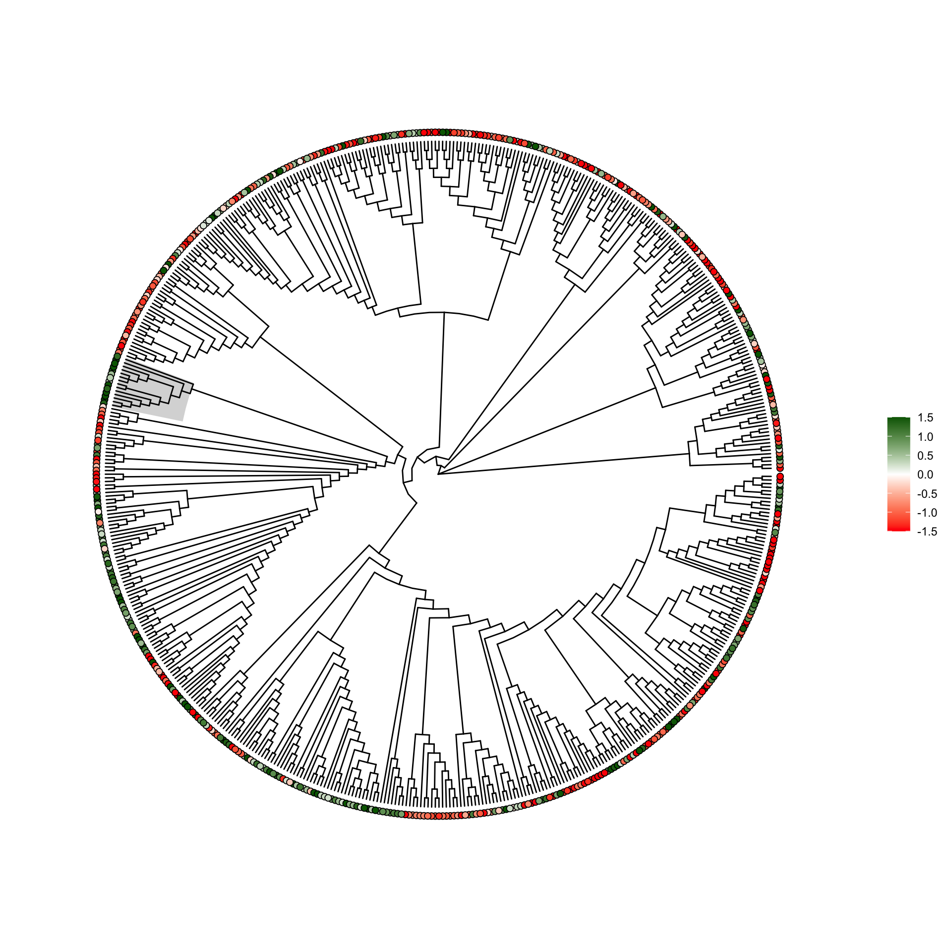
Maybe save it instead of plotting it in R.:
ggsave('cladogramwithinference.pdf',g3,height = 20, width = 20)References
Xia, Yinglin, Jun Sun, and Ding-Geng Chen. Statistical analysis of microbiome data with R. Springer, 2018.